Graph drawings in TikZ.

February 3, 2011

Kazimierz Kuratowski

Filed under: Uncategorized — fbc @ 01:00

It was just a day like yesterday, February 2, but from 1896 that the mathematician K. Kuratowski was born. Kuratowski proved in 1930 a theorem that characterizes planar graphs (graphs that can be drawn in a sheet of paper with no pair of edges crossing each other). The theorem states that a graph is planar if and only if it does not “contain” a copy of the complete bipartite graph K_{3,3} or of the complete graph K_5. We now show the two drawings corresponding to the graphs mentioned in the theorem.

Kuratowski graphs

Forbidden graphs

Pdf version of the drawing.

If we look at the picture carefully we may notice that it appears that edges are one on top of the other. To achieve this we used the following definitions (macros) in the preamble of our document.

\tikzstyle myBG=[line width=3pt,opacity=1]

\newcommand{\drawLinewithBG}[2]
{
  \draw[white,myBG]  (#1) -- (#2);
  \draw[black,very thick] (#1) -- (#2);
}
\newcommand{\drawPolarLinewithBG}[2]
{
  \draw[white,myBG]  (#1) -- (#2);
  \draw[black,very thick] (#1) -- (#2);
}

The commands we just defined tell TikZ to first draw a white line whose width is 3pt and then draw a black line on top of the white one.

The TikZ code that generates the drawing is the follwing.

\begin{tikzpicture}

  \useasboundingbox (-6.5,-3) rectangle (5.5,3);

  \begin{scope}[xshift=-6cm,yshift=-1cm]
    \foreach \x in {4,2,0} {
      \foreach \y in {0,2,4} {
        \drawLinewithBG{\x,0}{\y,2};
      }
    }

    \foreach \x in {0,2,4} {
      \foreach \y in {0,2} {
        \node at (\x,\y) [circle,fill=black] {};
      }
    }

    \node at (2,-1.5) {\Large$K_{3,3}$};
  \end{scope}

  \begin{scope}[xshift=3cm]
    \foreach \a in { 18, 90, 162, 234, 306 } {
      \foreach \b in { 18, 90, 162, 234, 306 } {
        \drawPolarLinewithBG{\a:2}{\b:2};
      }
    }

    \foreach \a in {18,90, 162, 234, 306 } {
      \node at (\a:2cm) [circle,fill=black] {};
    }
    \node at (0,-2.5) {\Large$K_5$};
  \end{scope}

\end{tikzpicture}

Until next time!

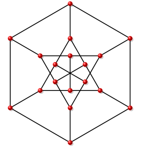
June 5, 2010

Pappus Graph

On the occasion of the 84 anniversary of the birth of Claude Berge, who formulated the Strong Perfect Graph Conjecture, we present a drawing of a perfect graph, the Pappus graph.

Pappus Graph

Pappus Graph

The drawing in pdf format.

This time, we just used the shadows library from TikZ.

\usetikzlibrary{shadows}

The source code that generates this drawing is

\begin{tikzpicture}[
vertex_style/.style={circle,shading=ball,ball color=red,draw=red!80!white,drop shadow={opacity=0.4}},
edge_style/.style={ultra thick, black,drop shadow={opacity=0.4}}]

\useasboundingbox (-5.05,-5.3) rectangle (5.1,5.25);

\begin{scope}[rotate=90]
   \foreach \x/\y in {0/1,60/2,120/3,180/4,240/5,300/6}{
      \node[vertex_style] (\y) at (canvas polar cs: radius=2.5cm,angle=\x){};
   }
   \foreach \x/\y in {0/7,60/8,120/9,180/10,240/11,300/12}{
      \node[vertex_style] (\y) at (canvas polar cs: radius=5cm,angle=\x){};
   }

   \foreach \x/\y in {0/13,60/14,120/15,180/16,240/17,300/18}{
      \node[vertex_style] (\y) at (canvas polar cs: radius=1.25cm,angle=\x){};
   }

\end{scope}

\foreach \x/\y in {13/16,14/17,15/18}{
   \draw[edge_style] (\x) -- (\y);
}

\foreach \w/\x/\y/\z in {1/7/14/18,2/8/15/13,3/9/16/14,4/10/17/15,5/11/18/16,6/12/13/17}{
   \draw[edge_style] (\w) -- (\x);
   \draw[edge_style] (\w) -- (\y);
   \draw[edge_style] (\w) -- (\z);
}

\foreach \x/\y in {7/8,8/9,9/10,10/11,11/12,12/7}{
   \draw[edge_style] (\x) -- (\y);
}
\end{tikzpicture}

May 14, 2010

Tutte’s Graph

Filed under: Graphs — fbc @ 22:41
Tags: , , , , ,

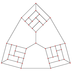
On the occasion of the 93 anniversary of the birth of William Tutte, we present a drawing of Tutte’s graph.

Tutte's Graph

Tutte

The pdf file.

As in our previous example, we used the shadows library from TikZ.

\usetikzlibrary{shadows}

Now, the code that generates the drawing.

\begin{tikzpicture}[
 vertex_style/.style ={circle,shading=ball,ball color=red,draw=red!40!white,drop shadow={opacity=0.4}},
 edge_style/.style={ultra thick, black},rotate=-30]

 \useasboundingbox (-14.2,-10.5) rectangle (14.3,16.2);

 \draw[edge_style] (0,0) -- (4.3431,0);
 \draw[edge_style] (0,0) -- (-2.1715,3.7612);
 \draw[edge_style] (0,0) -- (-2.1715,-3.7612);

 \draw[edge_style] (10,-5.6568) -- (-0.1010,-11.4886);

 \draw[edge_style] (-9.8989,5.8318) -- (-9.8989,-5.8318);

 \draw[edge_style] (10,5.6568) -- (-0.1010,11.4886);

 \node[vertex_style] at (0,0) {};
 % absolute positions
 \def\nodepos{0/0/0,1/0/2,2/4/2,3/4/4,4/0/4,
 5/-2/4,6/-4/4,7/-4/-4,8/4/-4,9/4/-2,
 10/4/0,11/2/0,12/2/-2,13/-2/-2,14/-2/0}

 \begin{scope}[rotate=0,xshift=10cm,rotate=135]
 \foreach \n/\x/\y in \nodepos{ \coordinate (\n) at (\x,\y);}
 \end{scope}

 \draw[edge_style] (0)
 \foreach \x in {1,...,14}{ --(\x)} -- cycle;

 \foreach \x/\y in {0/11,1/4,2/10,5/14,7/13,9/12}{
 \draw[edge_style] (\x) -- (\y);
 }

 \foreach \x in {0,1,...,14}{
 \node[vertex_style] at (\x){};
 }

 \begin{scope}[rotate=120,xshift=10cm,rotate=135]
 \foreach \n/\x/\y in \nodepos{ \coordinate (\n) at (\x,\y);}
 \end{scope}

 \draw[edge_style] (0)
 \foreach \x in {1,...,14}{ --(\x)} -- cycle;

 \foreach \x/\y in {0/11,1/4,2/10,5/14,7/13,9/12}{
 \draw[edge_style] (\x) -- (\y);
 }

 \foreach \x in {0,1,...,14}{
 \node[vertex_style] at (\x){};
 }

 \begin{scope}[rotate=240,xshift=10cm,rotate=135]
 \foreach \n/\x/\y in \nodepos{ \coordinate (\n) at (\x,\y);}
 \end{scope}

 \draw[edge_style] (0)
 \foreach \x in {1,...,14}{ --(\x)} -- cycle;

 \foreach \x/\y in {0/11,1/4,2/10,5/14,7/13,9/12}{
 \draw[edge_style] (\x) -- (\y);
 }

 \foreach \x in {0,1,...,14}{
 \node[vertex_style] at (\x){};
 }

\end{tikzpicture}

Until next time!
April 17, 2010

Petersen Graph

Filed under: Graphs — fbc @ 21:52
Tags: , , , ,

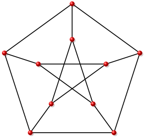
On the occasion of the 303 anniversary of the birth of  Leonhard Euler, father of graph theory, we start publishing this week in this blog. We now show a drawing of the Petersen graph.

The Petersen Graph

Picture of the Petersen graph

The drawing in pdf format.

To generate the vertex and edge shadows in this diagram we have used the shadows library from TikZ. We suggest to include the following line in the preamble of the document.

\usetikzlibrary{shadows}

We now show the TikZ code we used to generate this drawing.

\begin{tikzpicture}[
vertex_style/.style={circle,shading=ball,ball color=red,draw=red!80!white,drop shadow={opacity=0.4}},
edge_style/.style={ultra thick, black,drop shadow={opacity=0.4}}]

\useasboundingbox (-5.05,-4.4) rectangle (5.1,5.25);

\begin{scope}[rotate=90]
 \foreach \x/\y in {0/1,72/2,144/3,216/4,288/5}{
 \node[vertex_style] (\y) at (canvas polar cs: radius=2.5cm,angle=\x){};
 }
 \foreach \x/\y in {0/6,72/7,144/8,216/9,288/10}{
 \node[vertex_style] (\y) at (canvas polar cs: radius=5cm,angle=\x){};
 }
\end{scope}

\foreach \x/\y in {1/6,2/7,3/8,4/9,5/10}{
 \draw[edge_style] (\x) -- (\y);
}

\foreach \x/\y in {1/3,2/4,3/5,4/1,5/2}{
 \draw[edge_style] (\x) -- (\y);
}

\foreach \x/\y in {6/7,7/8,8/9,9/10,10/6}{
 \draw[edge_style] (\x) -- (\y);
}
\end{tikzpicture}

Until next week!

Create a free website or blog at WordPress.com.